
Institutional investors have portfolios worth hundreds of billions of dollars, this means that every position they need to liquidate will have an impact on the market price, since the quantity demanded at the highest bid price is not enough to absorb the position liquidated and so it will take place at different prices. This should be considered even when calculating risk measures such as VaR or the Expected Shortfall, because the value of the position needs to be adjusted for the real price at which it will be liquidated.

What is liquidity?
First we are going to briefly introduce what is intended with “liquidity”. It represents the trade off we have between how quickly we can sell an asset and how much the price of the asset is affected by the transaction. This is what it’s called “market liquidity”. It could be measured over three dimensions:
Width: which is the bid-ask spread
Depth: measures the quantity of securities that can be bought before influencing the price
Resiliency: measures the time needed to go back to the original price

To compute the liquidity for a certain security we can introduce the Liquidity Index (LIX). It comes from a work of Oleh Danyliv, Bruce Bland, Daniel Nicholass (2014) and is used to compute the amount of money needed to produce a daily single unit price fluctuation of the stock and the formula for this is:

Where Vt is the trading volume today, Pmid,t is the average of ask price and bid price, Phigh,t is the highest ask price today and Plow,t is the lowest bid price today. The logarithm is needed to reduce the interval of the results and ranges from 5, which is a very illiquid market, to 10, which is very liquid.
Optimal execution of orders
How may liquidity risk be included in a risk management model?
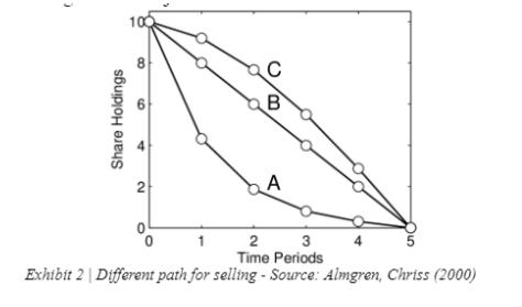
The work of Almgren and Chriss, who in 2000 established an optimal trade execution model that accounts for price impact as well as market risk, provides some hints. The model tries to reduce costs brought on by price impact as well as price risk (Almgren and Chriss 2000). They came up with the best stock trading execution tactics by minimizing a quadratic utility function under the assumption of a straightforward linear market impact model.
The market impact cost is the cost incurred by the trader due to the impact of their trades on the market, which can cause the prices to move against them. The risk cost is the cost incurred by the trader due to the risk of holding the portfolio during the execution period. The Almgren-Chriss model uses a dynamic programming approach to solve the optimization problem. It breaks down the execution period into small time intervals and determines the optimal trading strategy for each interval based on the current market conditions and the trader's objectives. The model also takes into account the trader's information about the market, such as the bid-ask spread and the volume at each price level.
For example if you received a signal that the price is going down and you are going to sell too fast you will have higher transaction costs, but lower uncertainty about the future price of the security, while trading in small transaction will have less impact on the market, but it will have higher uncertainty, so the question is: which is the optimal strategy? The model we are going to present is valid for discrete time, there is also a continuous time model, even with different assets, but it is far more complex to present and requires really good knowledge of the subject.
The factors considered in this model are:
Time: where t0 = 0 and tn = Nt = T
Number of shares: where qn + 1 = qn - vn+1 x dt
Price: where Sn+1 = Sn + sigma x sqrt(dt) x epsilon n+1, so that the price follows a Random Walk
Cash: where Xn+1 = Xn + vn dt (Sn-f(vn)) so that f(vn)=n which represents that the more I sell, the more the price decreases
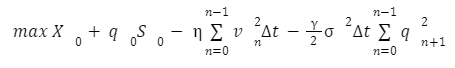
This problem can be resumed by an optimization of the function:

Which is a mean variance optimization problem, where represents the aversion of the individual. We will report just a couple of passages from the demonstration, but we will not go really in depth.
Starting from the equation

We then expand it and obtain:

Where represents the execution costs and the last term represents the noise, by selling faster the noise will be reduced. At this point we can return to our objective function.
That is equal to minimizing this convex function:

Applying the FOC we obtain:

Which has the solution:

This result is coherent, since for a more risk averse individual it recommends to go faster, while for a more illiquid market it recommends to go slower.
We presented this model to show that the value of a position should be adjusted for the cost of the transaction, since it is not possible to liquidate it at the current price, however it should be possible to find the strategy that has the highest expected value, considering the risk aversion of the investor.
Liquidity Adjusted VaR and Expected Shortfall
Usual VaR does not take into account liquidity risk, it assumes that the market has illimited depth, so the value of the position is overestimated, and is different from the realized liquidation. This is crucial when calculating ratios for stability of financial institutions, particularly for the ones who have large concentrated positions. The models that integrate the liquidity risk are divided into two types: endogenous and exogenous. The first ones assume that the size of the position matters for the market liquidity, however they are more difficult to implement, while exogenous models are more straightforward but less sophisticated.
One way of modeling VaR to account for market liquidity risk was proposed by Cont and Wagalath (2015) and it starts by considering a portfolio where the returns are random so that:

If we consider no market impact the value of a buy-and-hold portfolio with i shares of asset i, i=1…n will be:

Usually institutional investors, as we said before are subject to constraints to avoid level of leverage too high, this could be represented as Lmax so that before a stress situation the equity ratio will be VELmax. If a loss of l% happens then the ratio increases and if it exceeds this level the leverage constraint is no longer respected:

And a portion of the portfolio equal to what follows will be liquidated:

However if the position is large enough it will influence the price dynamics of the market so that:

In which D represents a liquidity parameter for the market depth of the asset. This equation divides the returns into a fundamental component and an endogenous one, which is self induced, that depends on the liquidity at the moment of deleveraging.
All the things we have just said should be seriously taken into account when analyzing the position of financial institutions and from this we can see that the VaR is not an absolute risk measure, because it underestimates the losses for market impacting positions, so we need to introduce a more specific type of VaR.
The liquidity adjusted Value at Risk is the sum of the VaR and the exogenous liquidity cost (ELC), this was proposed by Bangia, Diebold, Schuermann and Stroughair (1999). They modeled the transaction price as the mid price plus half of the proportional bid-ask spread.

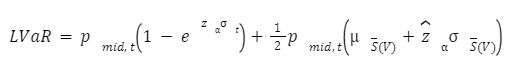
Where S is a time-varying proportional bid-ask spread. We can write the LVaR as it follows:

Where s is the volatility of daily returns, u is the mean of the proportional bid-ask spread, and z and z are the -percentile of the return distribution and the proportional spread distribution. This formula can be even made more precise by considering the Weighted Average Spread, which is a function of the volume of the stock in the portfolio and could be wrote as S(V).
Just to understand what is the real threat beneath the market liquidity constraint we take a look at this graph, which compares the size of a position with the difference between the VaR and the LVaR, and as we can see the LVaR increases exponentially as the position increases.

This opens another problem for institutions, since they need to evaluate which position they should liquidate first, should they liquidate smaller positions from different asset classes even if they are not losing money, or should they liquidate the most liquid position first? Surely the LVaR is less far from the traditional VaR for a more liquid asset. All these strategies should be included in the “living will” of the institution as a requirement of Basel III.

Comments