
Introduction
The concept behind the Phillips curve suggests that changes in the unemployment rate in the economy have a predictable impact on price inflation. The inverse relationship between unemployment and inflation is represented by a concave downward curve, with inflation on the Y axis and unemployment on the X axis. Rising inflation reduces unemployment and vice versa. Furthermore, prioritizing reducing unemployment also increases inflation and vice versa. In the 1960s, it was believed that any fiscal stimulus would increase aggregate demand and have the following effects. Demand for labor increases, the pool of unemployed workers then shrinks, and companies raise wages to compete and attract a smaller talent pool. Businesses' wage costs are increasing, and businesses pass these costs on to consumers in the form of price increases.
This belief system has led many governments to adopt a "backstop" strategy, in which a target inflation rate is set and fiscal and monetary policies are used to expand or contract the economy. economy to achieve the target rate. However, the stable trade-off between inflation and unemployment broke down in the 1970s with the rise of stagflation, calling into question the validity of the Phillips curve.

A paradigm shift
Stagflation occurs when an economy experiences stagnant economic growth, high unemployment, and high price inflation. Of course, this scenario directly contradicts the theory behind the Phillips curve. The United States never experienced stagflation until the 1970s, when rising unemployment did not coincide with falling inflation.
From 1973 to 1975, the US economy recorded six consecutive quarters of GDP decline, while inflation tripled. The phenomenon of stagflation and the breakdown of the Phillips curve have made economists more deeply interested in the role of expectations in the relationship between unemployment and inflation. Because workers and consumers can adjust their expectations of future inflation rates based on current inflation and unemployment rates, the inverse relationship between inflation and unemployment can only exist in the short term.
When the central bank increases inflation in order to push unemployment lower, it may cause an initial shift along the short-run Phillips curve, but as worker and consumer expectations about inflation adapt to the new environment, in the long-run, the Phillips curve itself can shift outward. This is especially thought to be the case around the natural rate of unemployment or NAIRU (Non Accelerating Inflation Rate of Unemployment), which essentially represents the normal rate of frictional and institutional unemployment in the economy. So in the long-run, if expectations can adapt to changes in inflation rates then the long-run Phillips curve resembles a vertical line at the NAIRU; monetary policy simply raises or lowers the inflation rate after market expectations have worked themselves out.
In the period of stagflation, workers and consumers may even begin to rationally expect inflation rates to increase as soon as they become aware that the monetary authority plans to embark on expansionary monetary policy. This can cause an outward shift in the short-run Phillips curve even before the expansionary monetary policy has been carried out, so that even in the short run the policy has little effect on lowering unemployment, and in effect, the short-run Phillips curve also becomes a vertical line at the NAIRU.

The model
Dwelving into the mathematics of the model we can summarize what we have just said with the formula proposed by Matheson and Stavrev (2013) model:
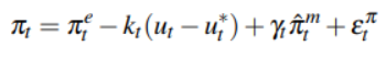
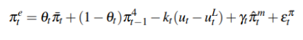
where πt is the consumer price index (CPI), πe is inflation expectations, ut is the unemployment rate, u∗ is the non-accelerating inflation rate of unemployment (NAIRU) t over the medium term, πˆm is the relative price of imports inflation, and επ is the cost t t push shock which are temporary one-time price jumps that do not continuously add to inflation overtime. For example, a one-time cost push is an increase in government expenditures shifting the overall demand in the economy when the economy is at full employment. The parameters, kt and γt, are assumed to be time-varying. In other words, the unemployment gap (ut − ut ∗) and import prices are not assumed to have a constant effect on inflation. Inflation expectations and the unemployment gap are treated as unobserved variables. Matheson and Stavrev (2013) assume the variables evolve as follows:

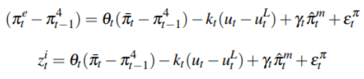
where π t is long run inflation expectations, πt−1 is year-over-year headline CPI inflation lagged one quarter. θt is the time-varying weight which is attached to long run inflation expectations and year-over-year inflation lagged one quarter. Matheson and Stavrev (2013) constrain θt between zero and one. The authors do this to show if πe has stabilized around the long run inflation target of the Federal Reserve. The existence of the unemployment gap, , is assumed to be constant and between 0 ≤ ≤ 1. In the first model we have two unknown parameters (k and u*), so it is impossible to solve the equation. However, to overcome this problem, we can assume u*t-1 as the NAIRU so we obtain:
where uL is the NAIRU. This model estimated by Matheson and Stavrev (2013) makes things difficult for us since its parameters are non linear, it would require an extended Kalman filter to solve the equation. However, as proposed by Matthew Burrell (2019) we can rewrite the equations in the following way in order to linearize the solutions and apply the Kalman filter:
The Kalman filter is a recursive algorithm that estimates the state of a dynamic system from a series of noisy measurements. It is a recursive algorithm, meaning that it updates its estimate of the state at each time step based on the previous estimate and the current measurement. The Kalman filter is also optimal in the sense that it minimizes the mean squared error of the estimate, it is based on a state-space model of the system. The state-space model describes the system`s dynamics and how the measurements are related to the state. The Kalman filter uses the state-space model to predict the next state of the system and to update its estimate of the state based on the current measurement. Here is a simplified example of how the Kalman filter works: suppose we are tracking a moving object. We can model the object's motion using a state-space model. The state of the object is its position and velocity. We can measure the object's position using a sensor, but the measurement is noisy. The Kalman filter uses the state-space model to predict the object's next position and velocity. It then updates its estimate of the object's position and velocity based on the current measurement. The Kalman filter also takes into account the uncertainty in the measurement noise. The Kalman filter repeats this process at each time step, resulting in an increasingly accurate estimate of the object's position and velocity.
A more detailed explanation of the Kalman filter could be found in our last research about Applying Kalman filter to pairs trading. To summarize, each vector of states can be expressed as a linear combination of the states in t-1, and this dependency can be found in the Gt matrix, which may vary over time, and a noise term (wt).
In matrices notation:
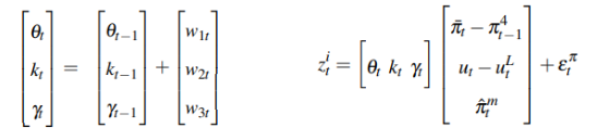
And:
The first equation on the left is called the equation of state which describes the dynamics of the state variables (Kim and Nelson, 1999). The dynamics of the state variables in this case are considered random walks. The state equation takes the form of a first-order differential equation in the state vector (Kim and Nelson, 1999). The second equation is called the measurement equation which describes the relationship between observed variables and the unobservable equation of state. wt and επ are disturbances that are assumed to be normally distributed and are assumed to be irrelevant at all lags.
Methodology
We took annual data for the CPI in the US, the natural rate of unemployment, the CPI change and the price inflation for all the commodities imported in the US from the FRED database and then we run the Kalman filter in order to iteratively estimate the parameters teta; k and gamma and we end up with the following graph. As we can see some parameters are less stable than other, however, we can clearly see that a static approach would reduce the explanatory power of this model.
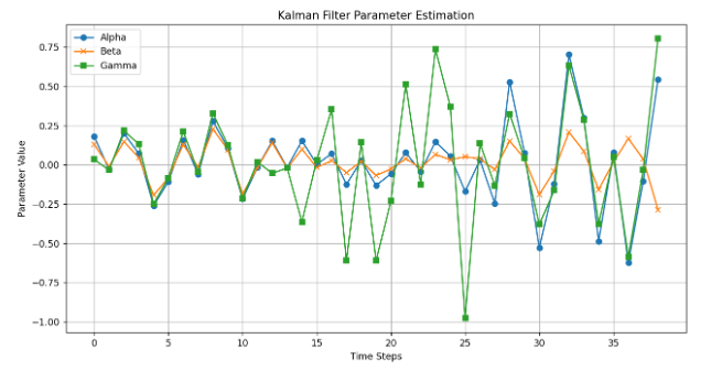
The time evolution of θ shows that the impact of inflation expectations on inflation during the 1960s until the 1980s, increases over time with several shocks to this parameter. By the early 1880s, this effect had diminished significantly. The downward increase can be attributed to the central bank's tightening monetary policy to combat inflation, which could lead to a change in inflation-related exceptions in the long run. During the 1990s, the impact of inflation expectations had less effect on inflation, which was surprising. One explanation for the results in the 1990s may be that the economy performed well during the Internet boom.
Next we can see that k can suggest that the Philips slope is not statistically significant because on average the effect of k will be close to 0. In other words, the time evolution of kt may be evidence that the usefulness of the Phillips curve in explaining inflation has diminished. For example, Atkeson and Ohanian (2001) and Levi and Makin (1980) question the usefulness of the relationship between the Phillips curve and inflation. Furthermore, these results are very different from Matheson and Stavrev (2013), where the slope evolution of the author's Phillips curve shows an increasingly coarser slope. Furthermore, the time evolution of the economy shows that during recessions, when unemployment rises, inflation rises when there should be deflationary pressure, which could mean that monetary policy does not work during recessions.
The time trajectory of γ was extremely variable between the 1990s and 2000s, and it is not possible to extract qualitative information from the graph. However, γ appears to have become extremely volatile again in the last few years. This can be explained by the fact that globalization has stabilized the impact of import prices on inflation in the United States, however many geopolitical factors have come into play (Covid and War). The impact of import prices during this period has a positive impact on inflation, meaning import prices contribute to increasing price pressure, as we saw with the rise in oil prices. Macroeconomic intuition is not as straightforward as one might expect regarding downward price pressures. The explanation for this result may be due to economic growth and the shift of production of goods abroad. In other words, income growth in the United States increases demand for manufactured goods around the world. Likewise, the price effect of imports has increased in recent years, which can be attributed to destabilization caused by tariffs imposed by the current US administration.
In addition, the influence of import prices has become more important since globalization in the 1990s. However, the slope of the Phillips curve remains questionable, so the usefulness of forecasting inflation using this model. Furthermore,
Matheson and Stavrev (2013) assumption of nonlinear parameters can be a reasonable argument that the estimation of kt over time is unreliable when using only a conventional Kalman filter.
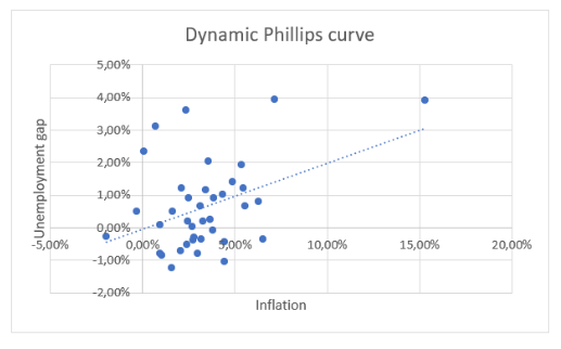
To further test if the model estimated would make sense we substituted in the general equation stated before the parameters we estimated and we solved for the expected inflation and then we plotted it against the unemployment to see if the tradeoff between growth and unemployment was respected and the results were nowhere near what we expected.
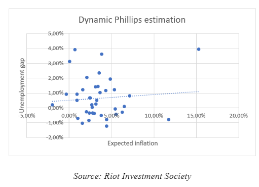
But then we made an hypothesis: since the translation of the unemployment gap into the inflation estimation process may take some time we tried lagging the inflation expectations by 1 and we obtained the following results, where it can clearly be seen that the tradeoff makes sense on average:
The positive relationship shown between the inflation estimations lagged and the unemployment gap confirms that as the unemployment gap increases the economy is overheating and it will need inflation to bring down purchasing power and salaries.
In conclusion the original assumption of the Phillips curve is not proven but it is not disproven either, however we can say that modeling the Phillips curve with a static approach is not optimal.

Comments